Newest
Topics:
For the latest news, see the NEWEST TOPICS page.
Google is too dumb to let me put the list of news in this column and falsely claims that all my pages are self-duplicates.
Google-NONSENSE
Google's so-called "Artificial Intelligence" is an abuse of the concept of intelligence!
Baro-acoustic decrepitation of Hall Mo samples,
Nevada
Using skew-gaussian curve fitting to determine
inclusion population parameters
Summary
By fitting gaussian component populations to the observed
baro-acoustic decrepitation data it is possible to derive
reproducible and precise temperatures for the individual
populations. Using the mode temperature of these component
populations it is possible to compare and contrast different
samples to assist mineral exploration and drill targeting.
These samples from the Hall deposit show quite complex
combinations of fluid inclusion populations, often with 5
components required to give a good fit to the data. Most samples
show a component with a temperature mode near 450 C as well as
about 550 C. Note that the peak at 580 to 590 C is related to
the alpha - beta quartz transition and is not used in
interpretation (explanation
here). A significant number of samples also have a
distinct component with a low mode temperature near or below 400
C. This separate low temperature component can be used to
classify the quartz into at least 2 types. Only sample 1188A had
visible molybdenite, which was abundant, but most if not all of
these samples are from potentially molybdenum bearing phases
according to Shaver's classification scheme.
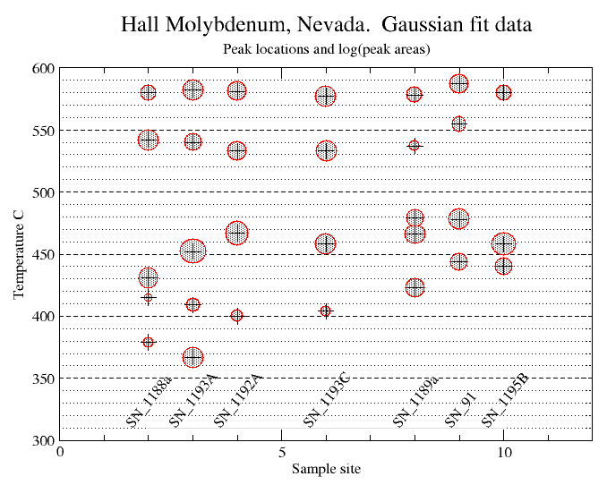
This plot summarises the individual fit results showing the
mode temperature of each component, with the size of the
peak (logarithmic area) represented by the circle diameter at
each plotted point. Note the presence of 350-400 C peaks
on the 4 leftmost samples, and the lack of this temperature on
the rightmost samples.
(Sample SN_91 on this plot is actually
SN_91-617)
This limited study of only 7 samples, together with the lack
of location information for some samples makes it impossible to
actually determine what decrepitation features might be used to
directly pinpoint mineralized quartz veins. However, the great
variations observed do suggest that fluid inclusion
decrepitation data within porphyry systems has the
potential to identify and outline features of importance which
could facilitate exploration.
Individual sample fitting results
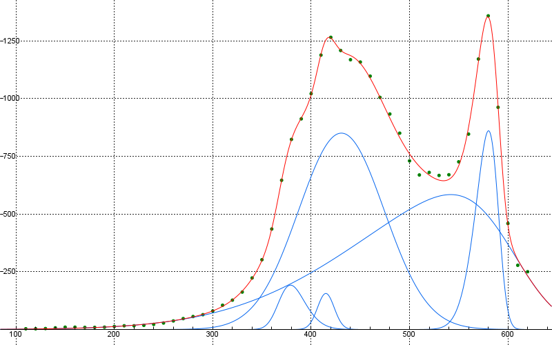
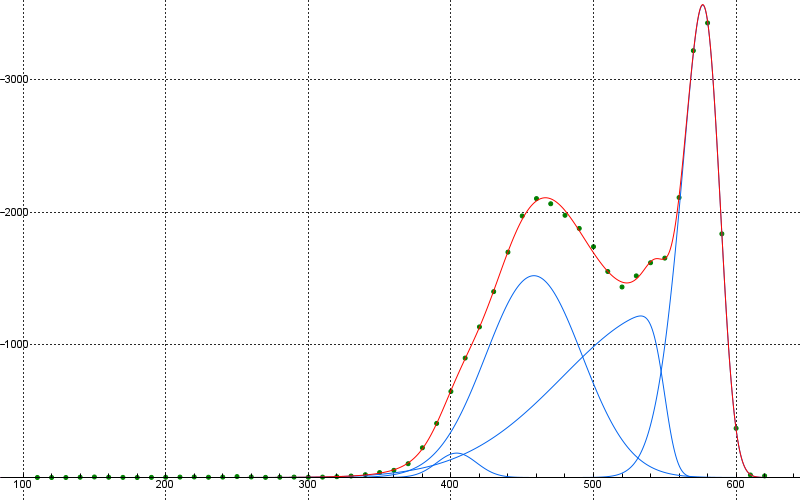
In these plots the green dots are the raw data points. The red
curve is the best fit sum of the component skew-gaussian curves,
each shown in blue. The "residuals" value indicates the goodness
of fit, with low values being a better fit to the raw data.
The curve fitting was done with the program fityk and the
summary plot was prepared with the program grace. (program information
here)
Sample 1188A, run G1644 5 peak fit, residuals=23. Sample
has low temperature components.
KQM1 zone, aplitic quartz monzonite, north stock, with abundant
molybdenite mineralization.
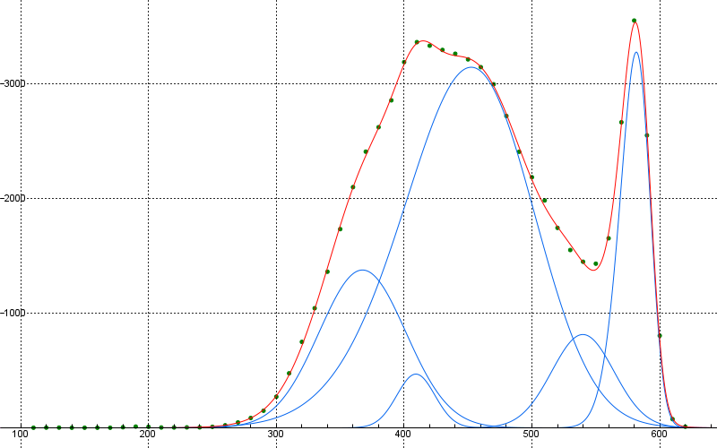
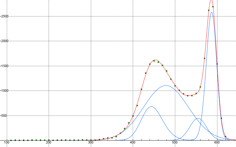
Sample 1193A run G1658 5 peak fit, residuals=54. Sample has a
very large and very low temperature component.
KC1 zone, chill zone of north stock. A molybdenite bearing phase,
but barren at the sample point.
NOTE: This is a subsample at the same location as G1661 below.
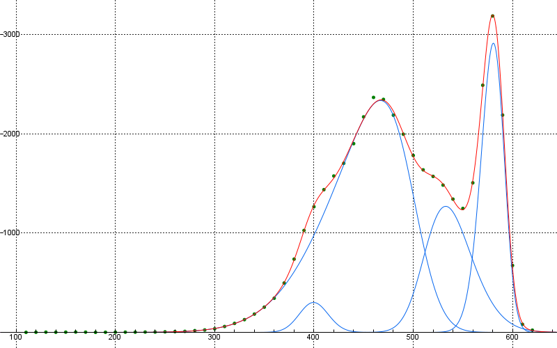
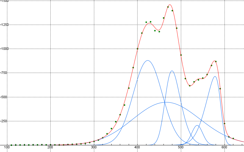
Sample 1192A run G1655 4 peak fit, residuals=28. Sample has a small
but distinct low temperature component.
Upper mine bench, sheeted quartz, north stock.
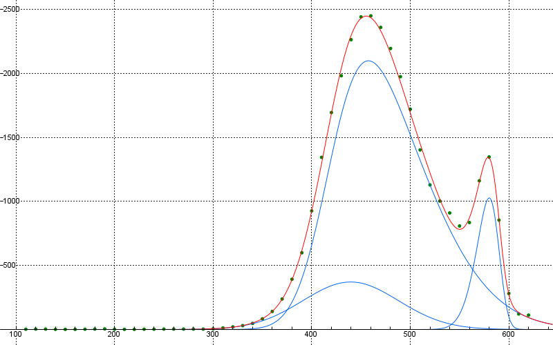
Sample 1193C run G1661 4 peak fit, residuals=54. Sample has only a
very small low temperature component.
KC1 zone, Chill zone of north stock. A molybdenite bearing phase,
but barren at the sample point.
NOTE: this is a subsample at the same location as G1658 above.
Sample 91-617 run G1544 4 peak fit, residuals=84. Sample has no low
temperature component.
Sample location and zone are unknown, sample was from Shaver's
museum collection.
Sample 1189A run G1646 5 peak fit, residuals=35. Sample has no low
temperature component.
South stock, upper mine bench, sheeted zone perimeter
Sample 1195B run G1668 3 peak fit, residuals=63. Sample has no low
temperature component.
KAP2 zone, aplitic porphyry, sheeted quartz zone of south stock
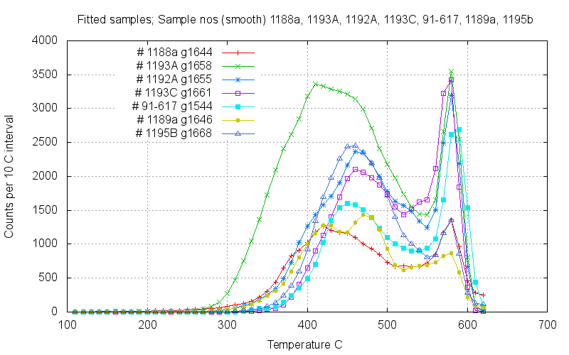
This plot shows the decrepitation results of all the above fitted
samples superimposed for comparison. The low temperature component
is visible on samples 1188a, 1193a and 1192a but it is not obvious
on 1193c, although the low temperature component was very small on
1193c. The other 3 samples had no low temperature component, but
without the gaussian fitting they cannot be easily distinguished on
this plot of unprocessed data.Samples 1193A (green) and 1193C
(magenta) are from the same location, but a few metres apart. They
give quite different decrepitation curves although they both have a
low temperature component population. This indicates that local
variability can be significant, perhaps because of overlap of
successive fluid events.
 Applied Mineral Exploration