Newest
Topics:
For the latest news, see the NEWEST TOPICS page.
Google is too dumb to let me put the list of news in this column and falsely claims that all my pages are self-duplicates.
Google-NONSENSE
Google's so-called "Artificial Intelligence" is an abuse of the concept of intelligence!
Resolving analytical histogram data into gaussian
component populations
A comparison of 3 different de-convolution programs.
Kingsley Burlinson
Introduction
The baro-acoustic decrepitation technique produces histograms of counts
versus temperature for each sample analysis. Each sample may contain
multiple populations of fluid inclusions which all contribute to the
overall histogram result. Although there have been suggestions made to
mathematically resolve the histogram (de-convolute) into its component
populations, this has not been easy to do. Recently, M.
Gibbes and M. Clark from Lismore University used de-convolution in
their study of
the hydrothermal deposits in the Drake district, NSW. In that work, the
decrepitation histograms were resolved into populations with a gaussian
distribution, but they found that using skewed gaussian distributions
for the populations gave better fits to the analytical data. They used
the software program PLOT,
for macintosh computers. The samples were de-convolved into many
individual populations, as many as 11 for each sample. Although
hydrothermal systems probably do contain very many different
populations of fluids, there is some concern that the large number of
components might be a mathematical artifact during the de-convolution.
And given this complexity, perhaps multiple re-fitting of the same data
using different software and operators might produce different results.
This discussion investigates the consistency and reproducibility of
de-convolution of decrepitation histograms performed using different
software packages and different operators over a one year period. One
specific sample was de-convolved numerous times, using 3 different
software packages. One de-convolution was performed using PLOT on
macintosh, 3 de-convolutions were performed using Scidavis on linux,
and 7 de-convolutions were performed using Fityk on linux.
Discussion
During their study of the Drake mineral field, NSW, Gibbes and Clark
collected 33 samples. One of these, sample number 28, from the Guy bell
pit is the object of this study. This sample was analysed by
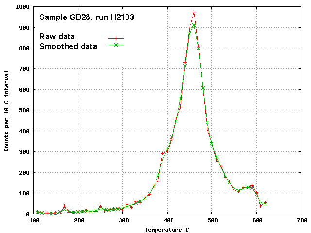
baro-acoustic decrepitation as analysis number H2133. The raw
analytical data was first smoothed using a weighted rolling mean of 3
samples and it is this smoothed decrepigram that was used for all the
mathematical de-convolutions. The unsmoothed data is shown below in
red, and the smoothed data in green.
Software program PLOT
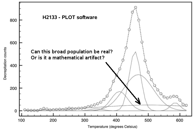
This software was used for one de-convolution by Gibbes and Clark,
reported in their published work (still in press) and shown below. They
resolved the data into 8 symmetrical gaussian populations. The
parameters for each population are not available and so the peak centre
(mode), peak height and peak width at half height were read off this
graph. Some interpolation was necessary and the values are necessarily
slightly imprecise. One of the populations in this de-convolution is
very wide, extending from 200 C to over 600 C. It is not clear if there
could actually be a fluid inclusion population with such a wide spread
of decrepitation temperatures. It could be caused if there were many
inclusions which have necked down, giving erratic and widespread
filling densities of the inclusions. But there is suspicion that this
population is an artifact of the mathematics rather than a real and
distinct fluid inclusion population.
Software program SCIDAVIS
Three de-convolutions were carried out using scidavis software.
This software does not include gaussian distributions by default, but
they can be added as a user created function. Although there is an
"auto-fit" function in this software, the starting values assumed fail
to lead to convergence and so the manual fit procedure must be used
with user entered starting values for each parameter. This often fails
to converge and repeated attempts with different starting parameters
may be required. It can be slow using this method, but it does work. In
addition, when using the manual fit procedure, the output plot does not
include a plot of each component population, only the final fitted
curve. To provide a complete plot it is necessary to use a custom
python script to read back in the fit parameters and add the
population curves to complete the plot. This custom script does make it possible to easily
save the individual curve parameters to an external file for additional
interpretation.
The deconvolutions were for 3 and 4 components using skewed
gaussian
populations and for 4 components using symmetrical gaussian
populations. It was not possible to achieve reasonable deconvolutions
using 5 components in this software as quite improbable populations
were generated for the fifth component. Once again, potentially
unrealistic broad
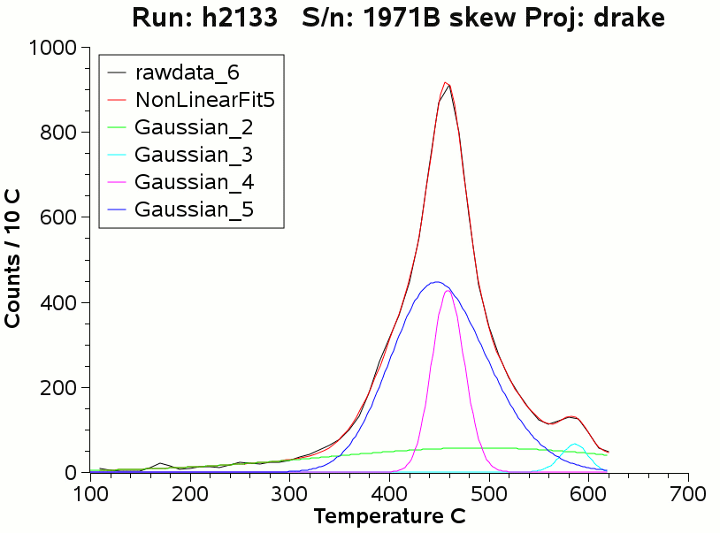
populations occurred in each fit (green). The 4 component skewed
gaussian fit
is better than the 4 component symmetrical gaussian fit, in accordance
with the
conclusion by Gibbes and Clark that skewed gaussian populations provide
a better de-convolution of the decrepitation data. The quality of fit
is given by the sums of squares of residuals divided by the degrees of
freedom (SSR/DoF) and lower values indicate a better fit to the input
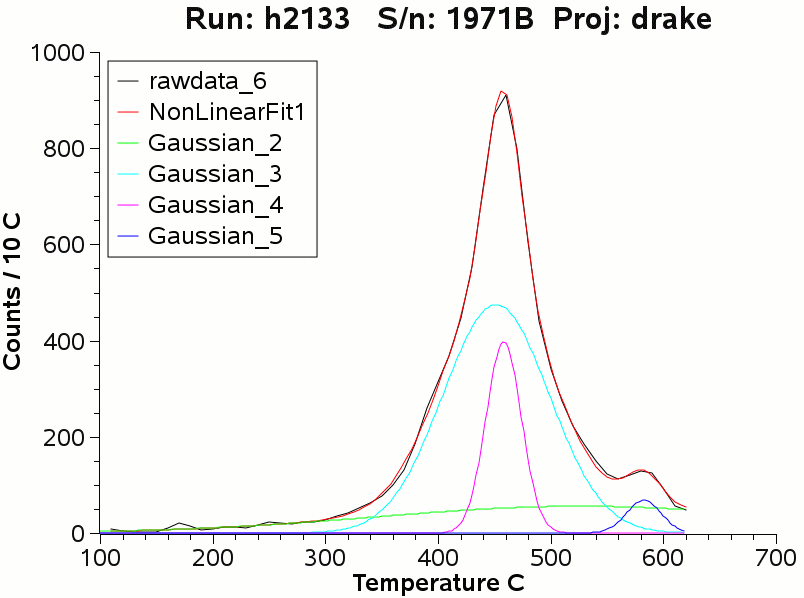
data. For the symmetrical gaussian populations, SSR/DoF was 40, while
for the skewed gaussian populations SSR/DoF was 26. Visually,
this improved fit is small, but noticeable, as seen in the next images
of the 2 types of fit.
The following image of the skewed gaussian fit shows a slightly better
match between the raw data (black) and the fitted sum curve (red). The
improvement is most noticeable between 520 C and 620 C.
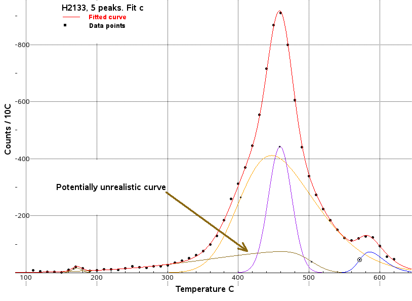
Software program Fityk
Seven fits were done using fityk, with 5 and 6 peaks, all populations
being skewed gaussian. This software has a convenient user
interface to allow the selection of peak positions and sizes visually
before performing the fit. It also has a simple scripting capability so
that the parameters of the fitted peaks can be easily exported to a
file. This program is widely used in the study of all types of spectra
from numerous analytical methods and it has an astonishing selection of
population shapes. Although the skewed gaussian population is not
present by default it can be added easily.
The fits for 5 populations all included a potentially unrealistic very
broad population, as seen here in brown in fit C. This broad population
is highly skewed. The SSR/DoF for this fit is 18, a very close fit, but
is it real?
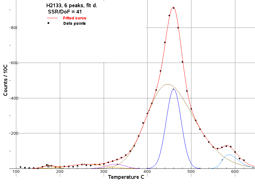
Attempts were made to achieve a fit which avoided a broad or highly
skewed component. Only one of the 7 fit attempts satisfied this
criteria. However fit D did not have a particularly low SSR/DoF value,
which was 41.
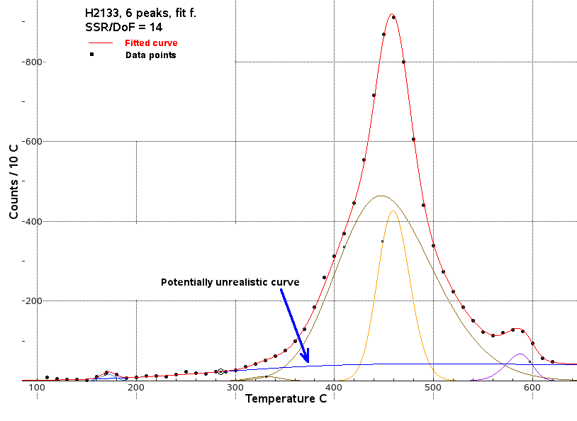
The lowest SSR/DoF value was 14 for fit F. However, this includes a
potentially unrealistic population (blue) with a very wide peak.
Despite the better SSR/DoF, this is not considered to be the best fit
because of this unrealistically broad component population. It was very
difficult to reach a convergence which did not include an unacceptably
broad population.
Comparison of the results from the different software packages.
For each fit performed with Scidavis and Fityk, the parameters for the
component populations were saved to an external file using some simple
scripts. This data is normally used to measure subtle differences
between samples in a full survey. But in this study, the results are
used to ascertain the stability and reproducibility of fits to the same
data set. The fit performed with PLOT software did not save these
parameters and it has been necessary to try and read these values from
the final plot which introduces some error.
Comparisons between results are normally done using the Mode
temperature for each peak. This is because the "central temperature"
used in the gaussian population formula does not occur at the maximum
height of the peak for skewed distributions. (The mode is the temperature at the peak of the curve.)
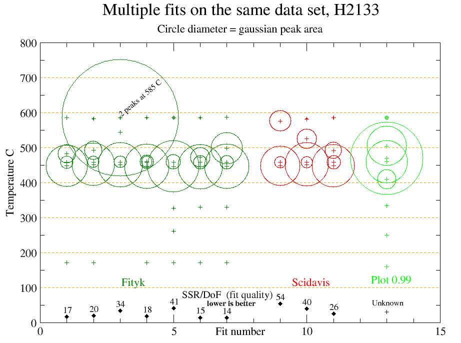
The temperature and width of each component population on each of the
11 fits in this study are plotted in the following X-Y-SIZE plots,
where the size of the plotted circle represents a linear function of
the area of the population peak. The area is merely an estimate and
calculated as Area = Constant *
peak_height * peak_width_at_half_height.
Although all the fits have a disturbingly broad peak, fit 3 (fityk, 5
peaks) and fit 13 (PLOT software, 8 peaks) have exceptionally broad
peaks which are of particular concern and are potentially unrealistic.
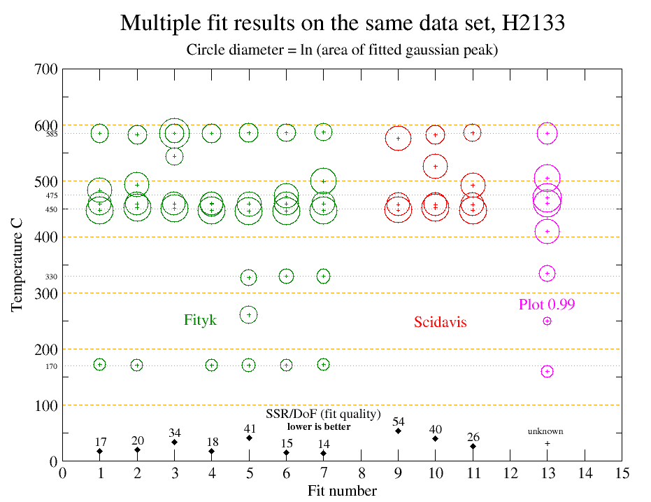
To compare variations in temperature between fits, the following plot
uses a natural logarithmic representation of the peak area. Additional
temperature grid lines highlight the differences between temperatures
of the fitted populations.
There are considerable differences between the multiple fits on this
single data set and clearly, de-convolution does not come close to
providing a unique or readily reproducible result. A significant
problem is due to the number of component populations. For fits using
3, 4, 5 and 6 populations, fityk and scidavis give the same pair of
peaks at about 450 C and 460 C. But PLOT, using 8 peaks, has these 2
peaks shifted higher to 460 C and 470 C. Fits 6 and 7, using fityk,
despite having almost identical and very good SSR/DoF values, have a
marked difference with fit 6 having a peak at 470C while fit 7 has this
peak at 500 C. Fit 10, by scidavis, has a peak at 525C which does not
match with any other fit. This fit used symmetrical gaussian
populations, which explains some of the difference, but fit 13 using
PLOT, also used symmetrical populations and did not locate a peak near
this temperature.
Conclusions
De-convolution of decrepigram curves does provide a way to compare
variations and similarities within a set of samples and is much more
precise than mere visual comparison of the decrepigrams. However,
de-convolution does not provide unique component population results and
there can be significant differences caused particularly by the choice
of how many peaks to include in the de-convolution. Visually, fits with
as few as 3 components give a close fit to the data. But as many as 8
peaks might be included if the software is allowed to automatically
choose the number of peaks to use.
A major concern is that many of the fit components have broad or very
skewed distribution shapes. Such populations are unlikely to be
physically realistic.
The performance of de-convolution depends on the nature of the raw
data, its noisiness and relative amplitudes. This particular study used
a sample with very low data values between 100 and 350 C which probably
exacerbated the fitting of this part of the curve.
The mathematically calculated component populations are only an aid in
the interpretation of the decrepigrams and are somewhat dependent on
operator choices. They should always be visually checked and critically
reviewed to ensure that the component populations are realistic. The
automatic fitting procedures in some software seem to have a tendancy
to produce very large numbers of component poulations in order to
achieve perfect fit. This may not be realistic, particularly if the
input data is slightly noisy.
 Applied Mineral Exploration