Analytical run h2284 of sample number 505a is from the Campbell's reef location.
In this plot, the yellow "Gaussian_6" plot is the mathematical sum of
the components and overlies the red "nonlinear fit" curve. This is
merely a confirmation that the deconvolution is correct. The 4
component populations provide a good match to the original "rawdata_6"
graph, but note that the peaks are visibly skewed rather than being
symmetrical gaussian distributions. This fit was done using the
Scidavis software package.
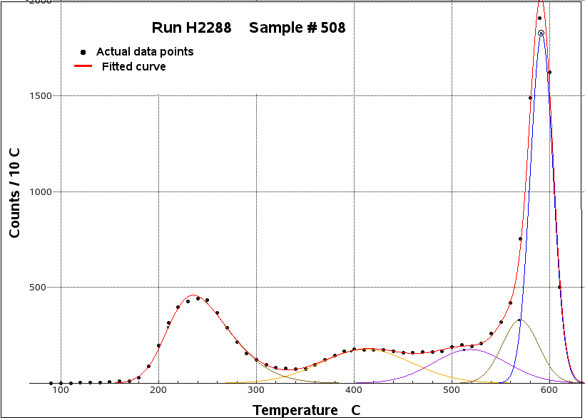
Analytical run h2288 of sample number 508 is from the 7 sublevel of the Morning Star mine.
In this fit, performed using the fityk software package, 5 populations
were required to provide a good fit to the raw data shown by the
unconnected filled circles. Note that 4 of the peaks are close to
symmetrical, while the low temperature peak at 240 C is moderately
skewed.
The details of the fitting procedure are discussed here.
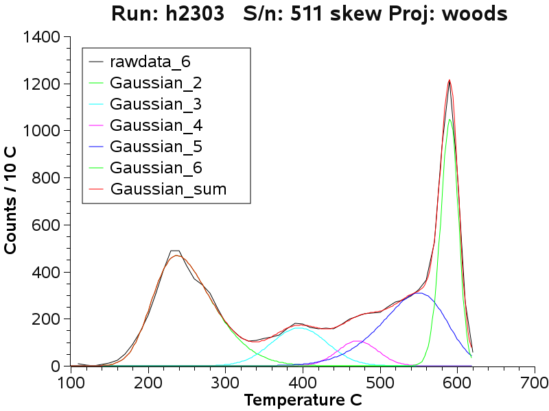
Analytical run h2303 of sample number 511 is from the Morning Star adit.
In this fit, 5 component populations provide a good fit to the raw data curve.
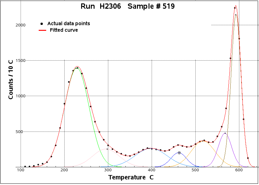
Analytical run h2306 of sample number 519 is from Dicken's reef.
In this fit 7 separate population components are required to provide a
good fit to the raw data. Note that all of the components are close to
symmetrical gaussian distributions.
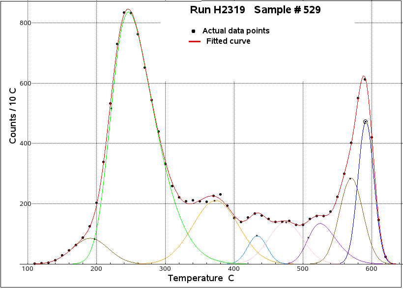
Analytical run h2319 of sample number 529 is from the 6 level of the Morning Star mine.
in this fit 8 component populations are required to fit the raw data.
Note the interesting additional low temperature peak at 190 C in
addition to the commonly observed population at 240 C. This indicates a
complex multiple stage deposition from fluids with significantly
different CO2 contents over time. This sample is thought to
contain 200 ppm of Au, one of the highest in the survey and perhaps
this additional CO2 peak is an especially favorable indicator for Au mineralisation potential. (Sample descriptions are here)
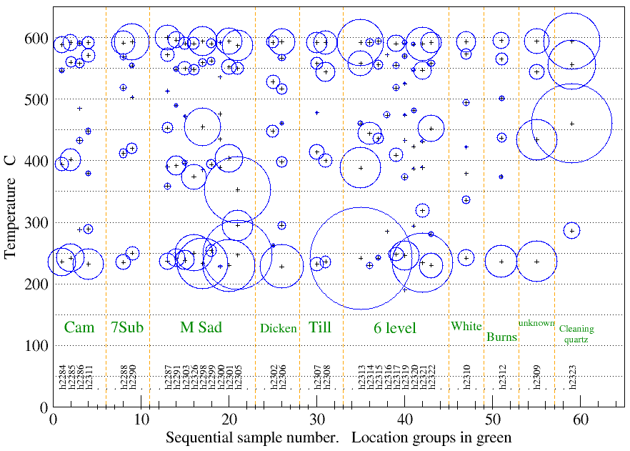
This plot shows the results of the peak fitting for all the samples in
this study. The mode temperature of each fitted population component is
shown by the black plus sign, with the radius of the blue circle around
each of these points being proportional to the height of the fitted
population peak. The most interesting feature is the presence of large
low temperature CO2 peaks in almost all of the samples.
Note that the cleaning quartz has a distinctly different low temperature peak.
Note also that sample h2319 (plotted at number 40) is the only sample with an additional low temperature peak at 190 C.
Conclusions:
The de-convolution of the decrepigrams provides a quantitative means to
compare and contrast the samples. It is best used within a spatial
suite of samples to define areas of similar mineralisation potential or
to discriminate between anomalous and background samples. The
complexity of the fits with many population components highlights the
known fact that hydrothermal systems are indeed complex with multiple
fluid events and they should not be thought of as simple homogeneous
events as they too often are merely because the quartz all looks the
same.
 Applied Mineral Exploration
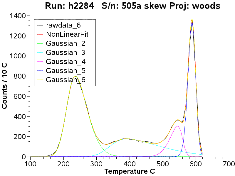
 The details of the fitting procedure are discussed here.